The Excel PMT (payment) Function is a really simple to use but highly useful Financial Function used to calculate the repayment amount on a loan. This function assumes that payments are made consistently (repayment frequency and amount remain constant) at a constant interest rate.
The video tutorial below will walk you through using the PMT Function (a full transcript of the video is below):
The PMT Function is used to calculate the payment required per period for loans based on constant payments at a constant interest rate. The periods themselves can be month, week or every two weeks. However, it must remain consistent with your payment period.
The PMT Function: =PMT(rate, nper, pv, [fv], [type])
The PMT Function requires:
It has two optional values:
The ‘Type’ lets you know whether the payment is going to be made on the first day of the month, or the last day of the month which is important for calculation of interest. You can use the future value function to allow you to calculate the payment required to meet a savings target.
Using the PMT Function:
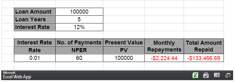
Here is a spread sheet we have set-up already with a number of values that we can use to calculate our payment amount.
(You can edit the values in the embedded Spreadsheet below to see how it works, or to download this spread sheet, click here)
The first thing that we need to do is calculate our interest amount for each of the months.
This particular repayment plan is going to happen on a monthly basis so we need to work out what the interest would be per month.
I take my interest rate (12% in cell C5) and divide it by 12 (number of months in a year). The Result is 0.01.
The number of payments over the lifetime of this loan would be 5 years (Loan Years in cell C4) multiplied by 12 which would give you 60 periods.
The present value, I can reference from cell F3 (i.e. $100 000). I can now calculate my PMT Function.
I reference my rate (cell B9), the number of periods (cell C9), and the present value(cell D9).
=PMT(B9, C9,D9)
Future Value and Type are in square brackets [] which mean these are optional parameters.
I now have my monthly repayment of -$2,224.44.
You’ll see that the value is represented as a negative value; this is because this is money going away from us in order to pay off this loan.
It will then be a simple matter to work out the entire amount paid for the life of the loan.
I take my monthly payment (cell E9) and multiply it by the number of payments that I need to make (cell C9).
=E9*C9 (The Result is -$133,466.69)
The PMT Function works if the interest rate is constant over the life of the loan and the period repayment plan is also constant for the entire life of the loan.
See Also: Sage 300 Tutorials and Demos